Create calendar with Excel formula and conditional formatting

We can build a calendar in Excel with only formula and conditional formatting.

  

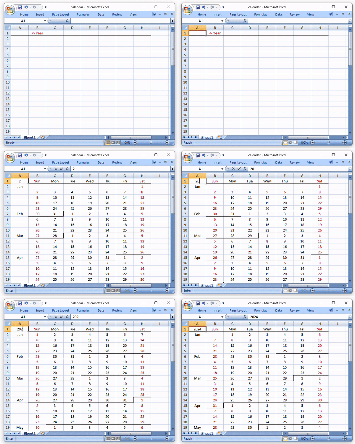
Year

Firstly type the year "2022" in cell A1.  You can type any year and the calendar will automatic update.

Day of Week Header

We use COLUMN() to get the day of week numeric value.

In cell B1, type the below formula and copy to B1:H1.

=TEXT(COLUMN()-1, "ddd")

Calendar Body

Then we fill the cells with the days count.

In cell B2, type the below formula and copy to B2:H55.

=(ROW()-2)*7+COLUMN()-1

and offset with day of week of 1-Jan, so "0" is 1-Jan, "1" is 2-Jan and so on.

=(ROW()-2)*7+COLUMN()-1-WEEKDAY(DATE($A$1,1,1))

Now we can construct the date by adding 1-Jan to the days count. Format the date to verify the formula is correct.

=TEXT(DATE($A$1,1,1)+(ROW()-2)*7+COLUMN()-1-WEEKDAY(DATE($A$1,1,1)),"yy-mm-dd")

Finally, we should only show date of current year, and the day of month instead of full date.

In cell B2, type the below formula and copy to B2:H55.

=IF(YEAR((DATE($A$1,1,1)+(ROW()-2)*7+COLUMN()-1-WEEKDAY(DATE($A$1,1,1))))=$A$1,DAY((DATE($A$1,1,1)+(ROW()-2)*7+COLUMN()-1-WEEKDAY(DATE($A$1,1,1)))),"")

Month Header

Next need to show the month in column A. If the row contains first day ("1") means it is a new month.  We can use MIN()=1 to determine if the row contains 1 instead of VLOOKUP(). And use TEXT(..., "mmm") to get the month name.

In cell A2, type the below formula and copy to A2:A55.

=IF(MIN(B2:H2)=1,TEXT(DATE($A$1,1,1)+(ROW(H2)-2)*7+COLUMN(H2)-1-WEEKDAY(DATE($A$1,1,1)),"mmm"),"")

Put everything together

We can put all three formula together. Apply the day of week formula in row 1, the month name formula in column 1. Also show a message in cell $A$2 if the year is not a number.

In cell A1, type the following formula and copy to A1:H55.

=IF(ADDRESS(ROW(),COLUMN())="$A$1","",IF(NOT(ISNUMBER($A$1)),IF(ADDRESS(ROW(),COLUMN())="$B$1","<- Year",""),IF(ROW()=1,TEXT(COLUMN()-1, "ddd"),IF(COLUMN()=1,IF(MIN($B1:$H1)=1,TEXT(DATE($A$1,1,1)+(ROW($H1)-2)*7+COLUMN($H1)-1-WEEKDAY(DATE($A$1,1,1)),"mmm"),""),IF(YEAR((DATE($A$1,1,1)+(ROW()-2)*7+COLUMN()-1-WEEKDAY(DATE($A$1,1,1))))=$A$1,DAY((DATE($A$1,1,1)+(ROW()-2)*7+COLUMN()-1-WEEKDAY(DATE($A$1,1,1)))),"")))))

Format

The calendar if half done now.  We need to add some format.

Select column A:H, apply the below formula in Conditional Formatting.

1. Add the bottom border as month separator if it is the first row (header) or the below is smaller that itself (i.e. next month)

=IF(ROW(A1)=1,TRUE,AND(COLUMN(A1)>1,A1<>"",A2<>"",A1>A2))

2. Add the right border as month separator in same row

=AND(COLUMN(A1)>1,ROW(A1)>1,A1<>"",B1=1)

3. Highlight Sat and Sunday to be red

=OR(COLUMN(A1)=2,COLUMN(A1)=8)

Finally , center align column A:H.  The calendar is done.

In addition, we can protect the worksheet and only allow to input the year.  Right click the cell A1, select "Format Cell", uncheck the "Locked" check box.

In menu "Review" -> "Protect Sheet".