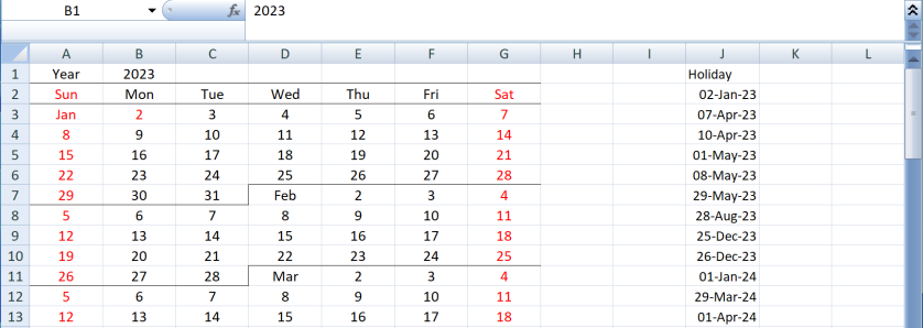
It is 2023 and I made an improved version of the Excel Calendar with a neat design and highlight the holidays.
Day of Week Header
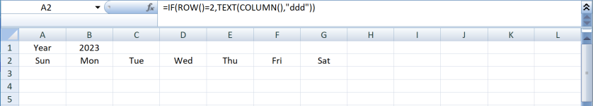
Firstly, input the year in cell $B$1 and create the day of week header. The day of week header only apply in row 2 and we use ROW() to ensure this.
In cell B1, type the below formula and copy to B1:H1
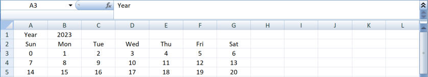
Day of the year
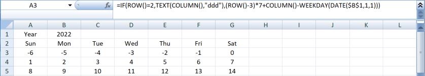
To construct the calendar, we fill up the cells with the day of the year (0-365). We need to offset by WEEKDAY(DATE($B$1, 1, 1) so day 0 fit in the correct day of week. It may not be easily noticed ince 1-Jan of 2023 is Sunday. It will be more clear if change the year to 2022.
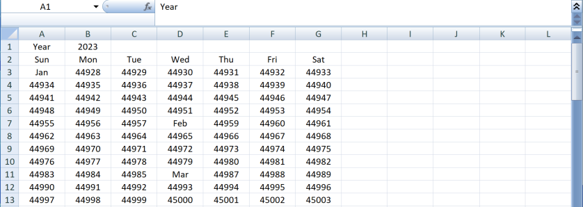
Date Value
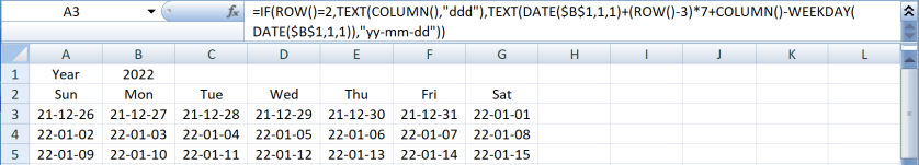
Now we add the first day of the year to to make it a date value so we can use conditional formatting to format it. Here we use TEXT() to format the date for verification only. This will be removed in actual formula.
Hide the date that does not match the input year.
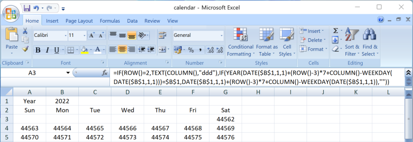
Fill up the worksheet
Copy the formula to cell A2:G55 to fill up the whole year
Format the calendar with Conditional Formatting
We then apply conditional formatting to format the calendar. Since the cell value is already a Date. We can use the date format to show the month name or day of month number.
Select column A:G and apply below Conditional Formatting:
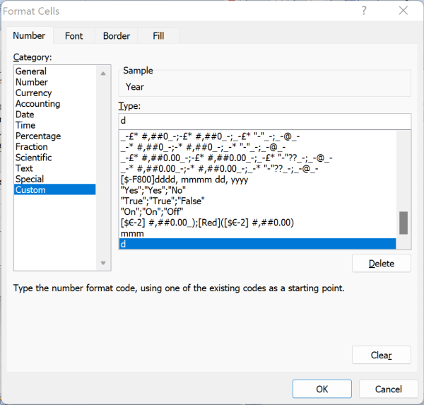
Show month name
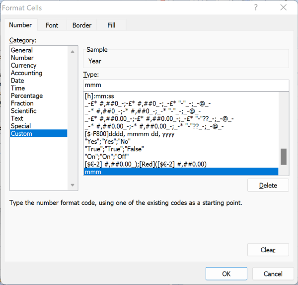
Use custom format mmm to show the month name in the first day of the month
Formula:
Format:
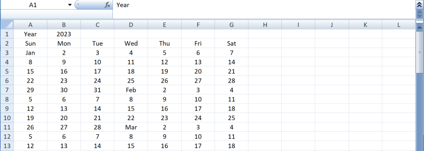
Number -> Custom -> "mmm"
Day number
Use custom format d to show the day number of remaining days of the month
Formula:
Format:
Border of month
Add a bottom border if reach end of the month (i.e. the day of month of next row is smaller than current cell
Formula
Format:
Border -> Bottom border
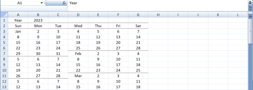
Add a right border for the last day of the month (i.e. the cell in the right is "1")
Formula
Format

Holiday
We highlight Saturday and Sunday in red. Also we can input the holiday and use Vlookup to mark the day as holiday as well.
Formula
Format
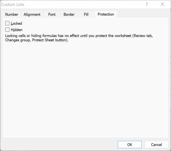
Protect Sheet
In last step, we unlock the cell $B$1 for input the year, and protect the worksheet